Note
You can download this demonstration as a Jupyter Notebook
here
Wealth transfer
This notebook presents a tutorial for beginners on how to create a simple agent-based model with the agentpy package. It demonstrates how to create a basic model with a custom agent type, run a simulation, record data, and visualize results.
[1]:
# Model design
import agentpy as ap
import numpy as np

# Visualization
import seaborn as sns
About the model
The model explores the distribution of wealth under a trading population of agents. Each agent starts with one unit of wealth. During each time-step, each agents with positive wealth randomly selects a trading partner and gives them one unit of their wealth. We will see that this random interaction will create an inequality of wealth that follows a Boltzmann distribution. The original version of this model been written in MESA and can be found here.
Model definition
We start by defining a new type of Agent with the following methods:
setup()is called automatically when a new agent is created and initializes a variablewealth.wealth_transfer()describes the agent’s behavior at every time-step and will be called by the model.
[2]:
class WealthAgent(ap.Agent):

    """ An agent with wealth """

    def setup(self):

        self.wealth = 1

    def wealth_transfer(self):

        if self.wealth > 0:

            partner = self.model.agents.random()
            partner.wealth += 1
            self.wealth -= 1
Next, we define a method to calculate the Gini Coefficient, which will measure the inequality among our agents.
[3]:
def gini(x):

    """ Calculate Gini Coefficient """
    # By Warren Weckesser https://stackoverflow.com/a/39513799

    x = np.array(x)
    mad = np.abs(np.subtract.outer(x, x)).mean()  # Mean absolute difference
    rmad = mad / np.mean(x)  # Relative mean absolute difference
    return 0.5 * rmad
Finally, we define our `Model <https://agentpy.readthedocs.io/en/stable/reference_models.html>`__ with the following methods:
setupdefines how many agents should be created at the beginning of the simulation.stepcalls all agents during each time-step to perform theirwealth_transfermethod.updatecalculates and record the current Gini coefficient after each time-step.end, which is called at the end of the simulation, we record the wealth of each agent.
[4]:
class WealthModel(ap.Model):

    """ A simple model of random wealth transfers """

    def setup(self):

        self.agents = ap.AgentList(self, self.p.agents, WealthAgent)

    def step(self):

        self.agents.wealth_transfer()

    def update(self):

        self.record('Gini Coefficient', gini(self.agents.wealth))

    def end(self):

        self.agents.record('wealth')
Simulation run
To prepare, we define parameter dictionary with a random seed, the number of agents, and the number of time-steps.
[5]:
parameters = {
    'agents': 100,
    'steps': 100,
    'seed': 42,
}
To perform a simulation, we initialize our model with a given set of parameters and call `Model.run() <https://agentpy.readthedocs.io/en/stable/reference_models.html>`__.
[6]:
model = WealthModel(parameters)
results = model.run()
Completed: 100 steps
Run time: 0:00:00.124199
Simulation finished
Output analysis
The simulation returns a `DataDict <https://agentpy.readthedocs.io/en/stable/reference_output.html>`__ with our recorded variables.
[7]:
results
[7]:
DataDict {
'info': Dictionary with 9 keys
'parameters':
    'constants': Dictionary with 3 keys
'variables':
    'WealthModel': DataFrame with 1 variable and 101 rows
    'WealthAgent': DataFrame with 1 variable and 100 rows
}
The output’s info provides general information about the simulation.
[8]:
results.info
[8]:
{'model_type': 'WealthModel',
 'time_stamp': '2021-05-28 09:33:50',
 'agentpy_version': '0.0.8.dev0',
 'python_version': '3.8.5',
 'experiment': False,
 'completed': True,
 'created_objects': 100,
 'completed_steps': 100,
 'run_time': '0:00:00.124199'}
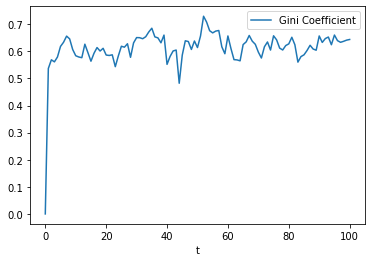
To explore the evolution of inequality, we look at the recorded `DataFrame <https://pandas.pydata.org/pandas-docs/stable/reference/api/pandas.DataFrame.html>`__ of the model’s variables.
[9]:
results.variables.WealthModel.head()
[9]:
| Gini Coefficient | |
|---|---|
| t | |
| 0 | 0.0000 |
| 1 | 0.5370 |
| 2 | 0.5690 |
| 3 | 0.5614 |
| 4 | 0.5794 |
To visualize this data, we can use `DataFrame.plot <https://pandas.pydata.org/pandas-docs/stable/reference/api/pandas.DataFrame.plot.html>`__.
[10]:
data = results.variables.WealthModel
ax = data.plot()
To look at the distribution at the end of the simulation, we visualize the recorded agent variables with seaborn.
[11]:
sns.histplot(data=results.variables.WealthAgent, binwidth=1);
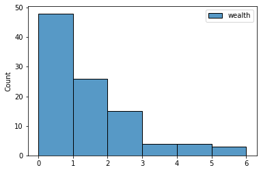
The result resembles a Boltzmann distribution.