Overview
This section provides an overview over the main classes and functions of AgentPy and how they are meant to be used. For a more detailed description of each element, please refer to the User Guides and API Reference. Throughout this documentation, AgentPy is imported as follows:
import agentpy as ap
Structure
The basic structure of the AgentPy framework has four levels:
The
Agentis the basic building block of a modelThe environment types
Grid,Space, andNetworkcontain agentsA
Modelcontains agents, environments, parameters, and simulation proceduresAn
Experimentcan run a model multiple times with different parameter combinations
All of these classes are templates that can be customized through the creation of sub-classes with their own variables and methods.
Creating models
A custom agent type can be defined as follows:
class MyAgent(ap.Agent):

    def setup(self):
        # Initialize an attribute with a parameter
        self.my_attribute = self.p.my_parameter

    def agent_method(self):
        # Define custom actions here
        pass
The method Agent.setup() is meant to be overwritten
and will be called automatically after an agent’s creation.
All variables of an agents should be initialized within this method.
Other methods can represent actions that the agent will be able to take during a simulation.
All model objects (including agents, environments, and the model itself) are equipped with the following default attributes:
modelthe model instanceida unique identifier number for each objectpthe model’s parameterslogthe object’s recorded variables
Using the new agent type defined above, here is how a basic model could look like:
class MyModel(ap.Model):

    def setup(self):
        """ Initiate a list of new agents. """
        self.agents = ap.AgentList(self, self.p.agents, MyAgent)

    def step(self):
        """ Call a method for every agent. """
        self.agents.agent_method()

    def update(self):
        """ Record a dynamic variable. """
        self.agents.record('my_attribute')

    def end(self):
        """ Repord an evaluation measure. """
        self.report('my_measure', 1)
The simulation procedures of a model are defined by four special methods that will be used automatically during different parts of a simulation.
Model.setupis called at the start of the simulation (t==0).Model.stepis called during every time-step (excluding t==0).Model.updateis called after every time-step (including t==0).Model.endis called at the end of the simulation.
If you want to see a basic model like this in action, take a look at the Wealth transfer demonstration in the Model Library.
Agent sequences
The Sequences module provides containers for groups of agents.
The main classes are AgentList, AgentDList, and AgentSet,
which come with special methods to access and manipulate whole groups of agents.
For example, when the model defined above calls self.agents.agent_method(),
it will call the method MyAgentType.agent_method() for every agent in the model.
Similar commands can be used to set and access variables, or select subsets
of agents with boolean operators.
The following command, for example, selects all agents with an id above one:
agents.select(agents.id > 1)
Further examples can be found in Sequences and the Virus spread demonstration model.
Environments
Environments are objects in which agents can inhabit a specific position. A model can contain zero, one or multiple environments which agents can enter and leave. The connection between positions is defined by the environment’s topology. There are currently three types:
Gridn-dimensional spatial topology with discrete positions.Spacen-dimensional spatial topology with continuous positions.
Applications of networks can be found in the demonstration models Virus spread and Button network; spatial grids in Forest fire and Segregation; and continuous spaces in Flocking behavior. Note that there can also be models without environments like in Wealth transfer.
Recording data
There are two ways to document data from the simulation for later analysis.
The first way is to record dynamic variables,
which can be recorded for each object (agent, environment, or model) and time-step.
They are useful to look at the dynamics of individual or aggregate objects over time
and can be documented by calling the method record() for the respective object.
Recorded variables can at run-time with the object’s log attribute.
The second way is to document reporters,
which represent summary statistics or evaluation measures of a simulation.
In contrast to variables, reporters can be stored only for the model as a whole and only once per run.
They will be stored in a separate dataframe for easy comparison over multiple runs,
and can be documented with the method Model.report().
Reporters can be accessed at run-time via Model.reporters.
Running a simulation
To perform a simulation, we initialize a new instance of our model type
with a dictionary of parameters, and then use the function Model.run().
This will return a DataDict with recorded data from the simulation.
A simple run can be prepared and executed as follows:
parameters = {
    'my_parameter':42,
    'agents':10,
    'steps':10
}

model = MyModel(parameters)
results = model.run()
A simulation proceeds as follows (see also Figure 1 below):
The model initializes with the time-step
Model.t = 0.Model.setup()andModel.update()are called.The model’s time-step is increased by 1.
Model.step()andModel.update()are called.Step 2 and 3 are repeated until the simulation is stopped.
Model.end()is called.
The simulation of a model can be stopped by one of the following two ways:
Calling the
Model.stop()during the simulation.Reaching the time-limit, which be defined as follows:
Defining
stepsin the paramater dictionary.Passing
stepsas an argument toModel.run().
Interactive simulations
Within a Jupyter Notebook, AgentPy models can be explored as an interactive simulation (similar to the traditional NetLogo interface) using ipysimulate and d3.js. For more information on this, please refer to Interactive simulations.
Multi-run experiments
The Parameter samples module provides tools to create a Sample
with multiple parameter combinations from a dictionary of ranges.
Here is an example using IntRange integer ranges:
parameters = {
    'my_parameter': 42,
    'agents': ap.IntRange(10, 20),
    'steps': ap.IntRange(10, 20)
}
sample = ap.Sample(parameters, n=5)
The class Experiment can be used to run a model multiple times.
As shown in Figure 1, it will start with the first parameter combination
in the sample and repeat the simulation for the amount of defined iterations.
After, that the same cycle is repeated for the next parameter combination.
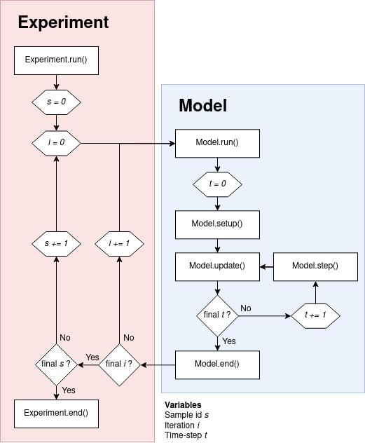
Figure 1: Chain of events in Model and Experiment.
Here is an example of an experiment with the model defined above. In this experiment, we use a sample where one parameter is kept fixed while the other two are varied 5 times from 10 to 20 and rounded to integer. Every possible combination is repeated 2 times, which results in 50 runs:
exp = ap.Experiment(MyModel, sample, iterations=2, record=True)
results = exp.run()
For more applied examples of experiments, check out the demonstration models Virus spread, Button network, and Forest fire. An alternative to the built-in experiment class is to use AgentPy models with the EMA workbench (see Exploratory modelling and analysis (EMA)).
Random numbers
Model contains two random number generators:
Model.randomis an instance ofrandom.RandomModel.nprandomis an instance ofnumpy.random.Generator
The random seed for these generators can be set by defining a parameter seed.
The Sample class has an argument randomize
to control whether vary seeds over different parameter combinations.
Similarly, Experiment also has an argument randomize
to control whether to vary seeds over different iterations.
More on this can be found in Randomness and reproducibility.
Data analysis
Both Model and Experiment can be used to run a simulation,
which will return a DataDict with output data.
The output from the experiment defined above looks as follows:
>>> results
DataDict {
'info': Dictionary with 5 keys
'parameters':
    'constants': Dictionary with 1 key
    'sample': DataFrame with 2 variables and 25 rows
'variables':
    'MyAgent': DataFrame with 1 variable and 10500 rows
'reporters': DataFrame with 1 variable and 50 rows
}
All data is given in a pandas.DataFrame and
formatted as long-form data
that can easily be used with statistical packages like seaborn.
The output can contain the following categories of data:
infoholds meta-data about the model and simulation performance.parametersholds the parameter values that have been used for the experiment.variablesholds dynamic variables, which can be recorded at multiple time-steps.reportersholds evaluation measures that are documented only once per simulation.sensitivityholds calculated sensitivity measures.
The DataDict provides the following main methods to handle data:
DataDict.save()andDataDict.load()can be used to store results.DataDict.arrange()generates custom combined dataframes.DataDict.calc_sobol()performs a Sobol sensitivity analysis.
Visualization
In addition to the Interactive simulations, AgentPy provides the following functions for visualization:
animate()generates an animation that can display output over time.gridplot()visualizes agent positions on a spatialGrid.
To see applied examples of these functions, please check out the Model Library.