Note
You can download this demonstration as a Jupyter Notebook
here
Interactive simulations
The exploration of agent-based models can often be guided through an interactive simulation interface that allows users to visualize the models dynamics and adjust parameter values while a simulation is running. Examples are the traditional interface of NetLogo, or the browser-based visualization module of Mesa.
This guide shows how to create such interactive interfaces for agentpy models within a Jupyter Notebook by using the libraries IPySimulate, ipywidgets and d3.js. This approach is still in an early stage of development, and more features will follow in the future. Contributions are very welcome :)
[1]:
import agentpy as ap
import ipysimulate as ips

from ipywidgets import AppLayout
from agentpy.examples import WealthModel, SegregationModel
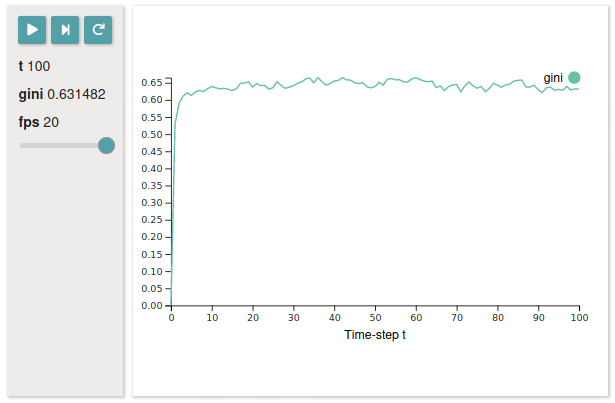
Lineplot
To begin we create an instance of the wealth transfer model (without parameters).
[2]:
model = WealthModel()
Parameters that are given as ranges will appear as interactive slider widgets. The parameter fps (frames per second) will be used automatically to indicate the speed of the simulation. The third value in the range defines the default position of the slider.
[3]:
parameters = {
    'agents': 1000,
    'steps': 100,
    'fps': ap.IntRange(1, 20, 5),
}
We then create an ipysimulate control panel with the model and our set of parameters. We further pass two variables t (time-steps) and gini to be displayed live during the simulation.
[4]:
control = ips.Control(model, parameters, variables=('t', 'gini'))
Next, we create a lineplot of the variable gini:
[5]:
lineplot = ips.Lineplot(control, 'gini')
Finally, we want to display our two widgets control and lineplot next to each other. For this, we can use the layout templates from ipywidgets.
[6]:
AppLayout(
    left_sidebar=control,
    center=lineplot,
    pane_widths=['125px', 1, 1],
    height='400px'
)
Note that this widget is not displayed interactively if viewed in the docs. To view the widget, please download the Jupyter Notebook at the top of this page or launch this notebook as a binder. Here is a screenshot of an interactive simulation:
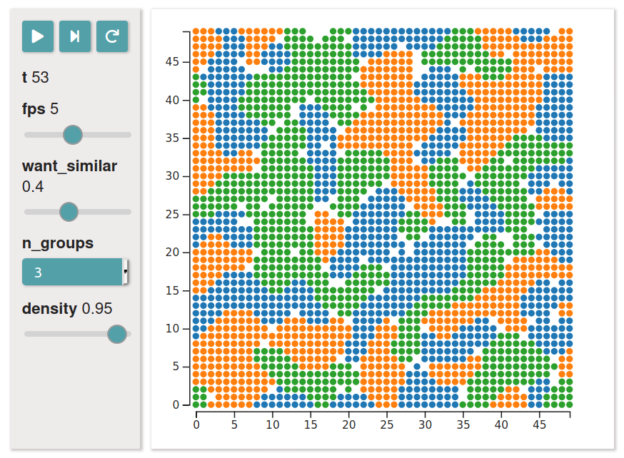
Scatterplot
In this second demonstration, we create an instance of the segregation model:
[7]:
model = SegregationModel()
[8]:
parameters = {
    'fps': ap.IntRange(1, 10, 5),
    'want_similar': ap.Range(0, 1, 0.3),
    'n_groups': ap.Values(2, 3, 4),
    'density': ap.Range(0, 1, 0.95),
    'size': 50,
}
[9]:
control = ips.Control(model, parameters, ('t'))
scatterplot = ips.Scatterplot(
    control,
    xy=lambda m: m.grid.positions.values(),
    c=lambda m: m.agents.group
)
[10]:
AppLayout(left_sidebar=control,
          center=scatterplot,
          pane_widths=['125px', 1, 1],
          height='400px')
Note that this widget is not displayed interactively if viewed in the docs. To view the widget, please download the Jupyter Notebook at the top of this page or launch this notebook as a binder. Here is a screenshot of an interactive simulation: